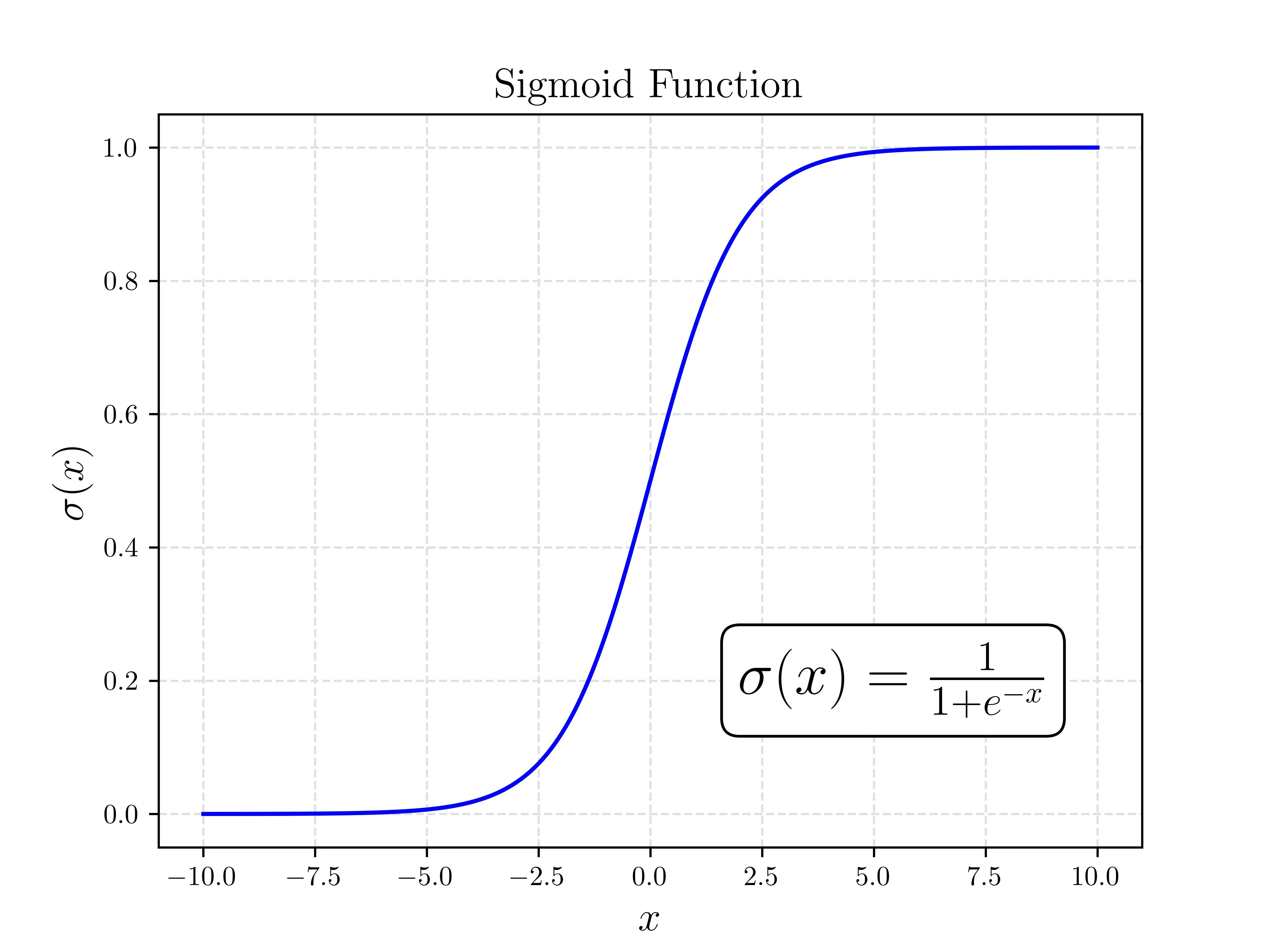
I’ve been getting some questions on how I created the sigmoid figure from my logistic regression post, in particular how I integrated LaTeX into matplotlib. It’s quite easy so I thought I’d share some tips and break down how I made that plot.
Prerequisites
Installing LaTeX
You’ll need to make sure that you have LaTeX intstalled on your computer. Many of us are used to using Overleaf so if you haven’t installed LaTeX locally I would start here.
Enabling LaTeX
Outside of your typical matplotlib imports you need to enable the rcParam text.usetex
import numpy as np
import matplotlib
matplotlib.rcParams['text.usetex'] = True
import matplotlib.pyplot as plt
%matplotlib inline

# Useful for running matplotlib on high-dpi displays
%config InlineBackend.figure_format='retina'
As an example, let’s build up the prior figure.
Creating Plot
Evaluating Sigmoid
Not that it’s relevant to LaTeX but the below was used to compute points for plotting.
X = np.linspace(-10, 10, int(1e3))
Y = 1 / (1 + np.exp(-X)) # Sigmoid function evaluated on X
And for generating the plot itself we’ll do go ahead and proceed in two steps.
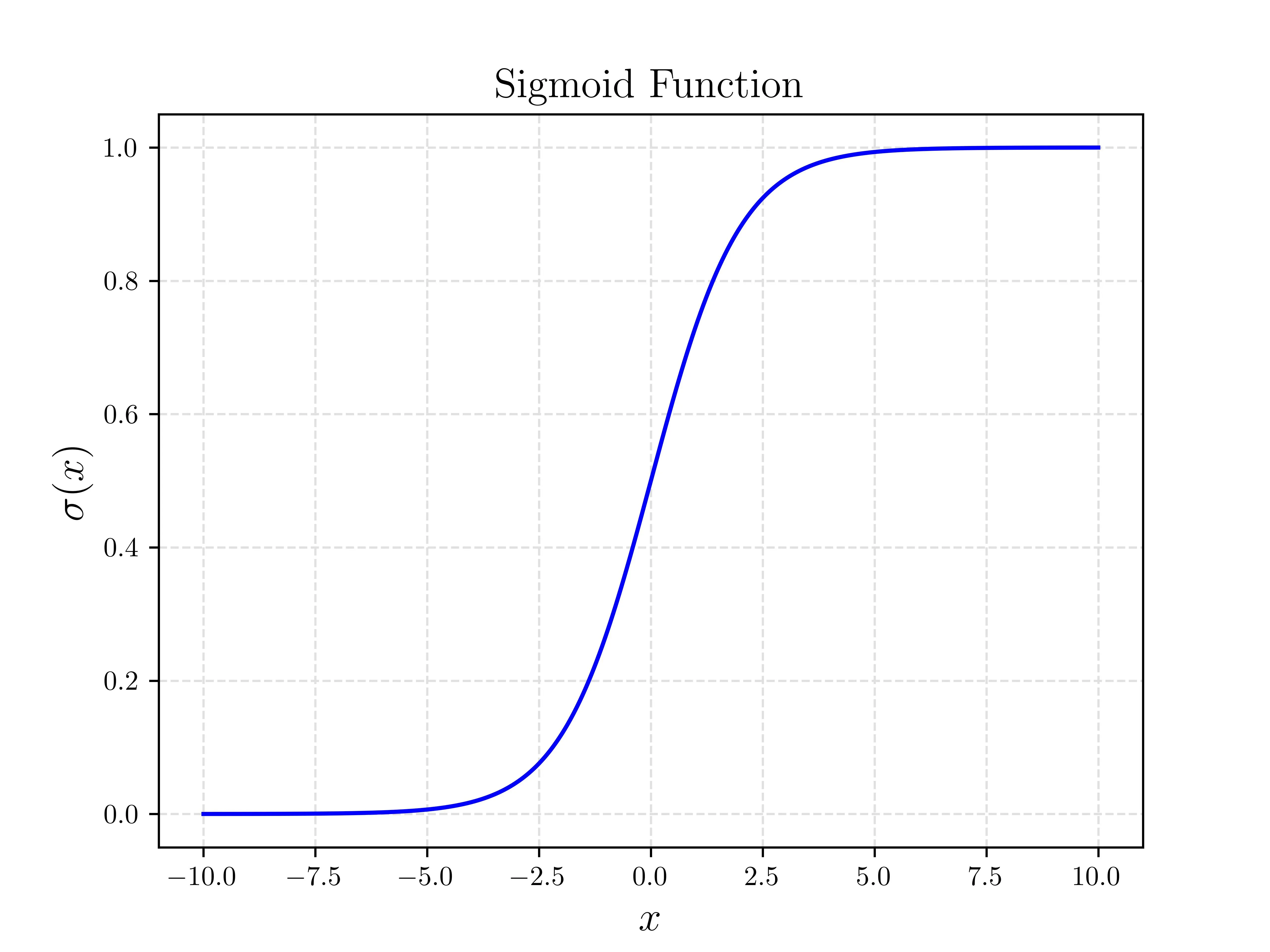
Primary Plot Axes
As you can see, to indicate you want to render a LaTeX equation all you need to do is pass a raw string with $$ around the equation in the LaTeX syntax.
plt.plot(X, Y, c='blue')
plt.title("Sigmoid Function",fontsize=15)
plt.xlabel(r"$x$", fontsize=15)
plt.ylabel(r'$\sigma(x)$', fontsize=15)
plt.grid()
plt.show()
This gives you the same plot you saw before without the written equation.
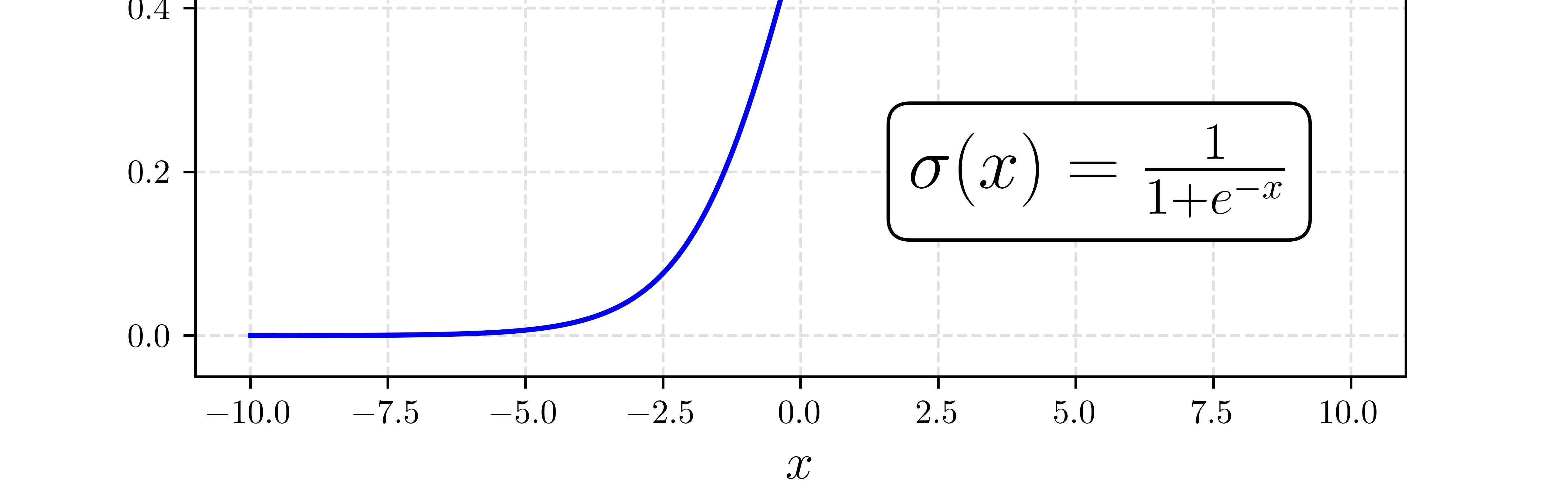
Equation Box
The equation box is a matplotlib text box with some additional specifiers for styling.
plt.text(2, 0.18, r'$\sigma(x)=\frac{1}{1+e^{-x}}$', fontsize=22,
         bbox=dict(boxstyle="round", ec=(0.0, 0.0, 0.0), fc=(1., 1, 1)))
Let’s go through the arguments to understand what’s going on here. Details here.
2, 0.18are the position argumentsr$...$is the input text, in this case an equationfontsizeis self-explanatorybboxis the style specifier.boxstyledetermines the bounding box styleecis a tuple of normalized RGB values for the border colorfcis the same asecexcept for fill color
With everything combined we get the original plot that is part of the original post.